CUDA Ray Tracing 2x Faster Than RTX: My CUDA Ray Tracing Journey
Introduction
Welcome! This article is a deep dive into how I made a CUDA-based ray tracer that outperforms a Vulkan/RTX implementation—sometimes by more than 3x—on the same hardware. If you're interested in GPU programming, performance optimization, or just want to see how far you can push a path tracer, you're in the right place.
The comparison is with RayTracingInVulkan by GPSnoopy, a well-known Vulkan/RTX renderer. My goal wasn't just to port Ray Tracing in One Weekend to CUDA, but to squeeze every last millisecond out of it—profiling, analyzing, and optimizing until the numbers surprised even me. And this is actually how I learned CUDA.
In this write-up, I'll walk you through the journey: what worked, what didn't, and the key tricks that made the biggest difference. Whether you're a graphics programmer, a CUDA enthusiast, or just curious about real-world GPU optimization, I hope you'll find something useful here.
Note
The original title claimed a 3.6x speedup, which was true at the time of writing — but after realizing I forgot to add Russian Roulette to RayTracingInVulkan, the performance difference shrunk to 2x. Still very significant, and it's more fair now.
| Renderer | Graphics API | Hardware Acceleration | Geometry Types | Performance (FPS) | GPU Time | Notes |
|---|---|---|---|---|---|---|
| RayTracingInVulkan (GPSnoopy) | Vulkan | RTX acceleration | Procedural sphere tracing + triangle modes | ~20 ms | ~50 FPS |
|
| CUDA-Ray-Tracing-In-One-Weekend(Mine) | CUDA | No hardware RT cores | Procedural spheres only | ~8 ms | 105 FPS |
|
Why is the Vulkan/RTX version slower? While there are many contributing factors, one likely explanation—pointed out by Tanguy Fautré (GPSnoopy)—the author of RayTracingInVulkan, shared his insights on why procedural ray tracing may underperform on NVIDIA RTX GPUs:
“My suspicion is that procedural spheres are relatively cheap to compute (both the ray intersection and shading), leaving the compute units mostly idling while the RT units are fully utilized doing BVH traversal. Thus the performance in this case is entirely limited by the RT units.
Interestingly, this article (and the Radeon RX 6900 XT results in RayTracingInVulkan procedural benchmarks, a GPU where the BVH traversal is handled by the compute units rather than its RT units) tend to support the idea that doing the entire BVH traversal using only the compute units is faster than delegating to the RT units. At least on the GeForce 3000 series and the Radeon RX 6000 series, that is.
In practice, the test scene is an unlikely scenario in gaming. In a modern AAA game, the compute cores will be actively used for shading and rendering the game, leaving little room on those units for doing the BVH traversal, while most (all?) of the ray intersections will be done against triangles (a task at which RT units excel, especially on later generation GPUs).”
Supporting this theory, RayTracingInVulkan consistently benchmarks better on AMD cards, such as the Radeon RX 6900 XT, which perform BVH traversal using compute units rather than dedicated RT hardware. This suggests that—at least on NVIDIA's 3000 series and AMD's 6000 series—doing everything in compute can outperform using fixed-function RT cores when the workload involves minimal shading and simple procedural intersections.
This also ties directly into NVIDIA's own guidance, which emphasizes that RT cores are architected to be most efficient with triangle geometry—not procedural primitives like spheres or AABBs:
“Use triangles over AABBs. RTX GPUs excel in accelerating traversal of AS created from triangle geometry.”
Of course, this is a synthetic scenario. In a typical AAA game, compute cores are heavily loaded with shading and post-processing tasks, and most ray intersections are against triangles—a case where RT cores excel, especially on newer generations of GPUs.
Another reason might be the ray tracing pipeline itself. While powerful and flexible, the hardware RT pipeline often incurs more overhead than inline ray tracing (Ray query). It tends to make heavy use of VRAM bandwidth by moving payload data around between shader stages. On the other hand, inline ray tracing can keep most of the data in registers, which is exactly what's happening in my implementation. So you can consider my approach as inline ray tracing This register-centric design drastically cuts down memory traffic and boosts performance.
So yes, it may sound like clickbait—but it's technically accurate, and when you dig into sample rates, shader complexity, geometry types, and hardware, the numbers hold up. In this article, I'll peel back the layers of how I squeezed 2x performance out through CUDA-level optimizations, giving you an exciting taste of what's possible when you really dig deep into cache behavior, register pressure, and GPU optimization.
Why CUDA?
As a graphics programmer, I'm constantly pushing the limits of what the GPU can do. But I realized that knowing just high-level shading languages or APIs like Vulkan or DirectX wasn't enough—I needed to understand the machine itself. CUDA gave me the lowest-level, most explicit way to explore how GPUs schedule threads, manage memory, and hit (or miss) performance targets. And with the help of Nsight Compute, I wasn't just reading theory—I was hands-on, exploring real bottlenecks, discovering how latency hiding works, learning about warp scheduling, cache behavior, and so much more. It introduced me to performance concepts I hadn't encountered before, and grounded them in actual numbers and experimentation.
And I didn't want to "just learn a language." I wanted to learn CUDA as a suite of tools, to really get under the hood of how GPU code runs, stalls, and gets optimized. So I asked myself: what's the best way to do that for a graphics programmer?
Answer: write a ray tracer from scratch in CUDA… and then squeeze it until it screams.
This article walks you through how I implemented a naive CUDA port of Ray Tracing in One Weekend that ran at 2.5 seconds per frame, and optimized it down to 9 milliseconds. Along the way, I hit every wall I could—scoreboard stalls, branching hell, memory layout issues—and learned how to knock each one down.
This isn't a language learning blog. It's an optimization story. A journey into how GPUs really work, and what it takes to make them fly.
And if you're into ray tracing, performance hacking, or just enjoy watching frame times drop—you're in the right place.
You can check out the source code along with it's commit history HERE.
Specifications:
To give proper context to the performance numbers and optimizations discussed in this article, it's important to understand the hardware I tested on. These specs shaped not only what was possible, but also where the real bottlenecks and wins emerged during tuning.
| Component | Specification |
|---|---|
| CPU | i5 13600KF |
| GPU | RTX 3080 10GB Desktop |
| CUDA Version | 12.9 |
| Resolution | 720x1280 |
| Samples | 30 |
| Max Ray Depth | 50 |
The Starting Point: A Naive CUDA Ray Tracer
Before any optimizations, I started with a direct CUDA port of Ray Tracing in One Weekend. No fancy tricks — just threads launching per pixel, tracing rays recursively plus traversing a BVH, so yes, we're already not even as slow as big O of N here.
And it worked. Technically. But it was slow — 2.5 seconds per frame kind of slow, slower than my old CPU version which was 1.5 seconds. Each thread handled one pixel, there was no memory layout optimization, and no thought given to how branching or recursion would behave on the GPU.
This was intentional. I wanted to start almost from zero, actually, from where I thought was fast last time I tried to optimize it :)
So with a chunky frame time and profiler in hand, I started breaking it down. Where was the time going? What was stalling? Why did a GPU that could chew through teraflops look like it was running on a potato?
Time to find out ... But first...
What CUDA Gives You (and What It Punishes You For)
CUDA is amazing because it gives you bare-metal control over how your code runs on the GPU. You're not writing shader code inside an engine or hoping a compiler figures things out — you're the compiler. You're the scheduler. You're the reason your app runs fast... or doesn't.
But with that power comes the traps. And the first trap I stepped into was recursion.
Recursion on the GPU sounds elegant — until you realize it's kryptonite for performance. Why?
- Register pressure: every level of recursion eats more registers, and once you're out, you're spilling to memory.
- Local memory access: spilled data goes to local memory, which is slow, and you don't get to control the layout.
- Stack usage: recursive calls build a big stack, and that stack sits in memory, not registers.
- Warp divergence: recursion usually means branching, and branching destroys SIMT efficiency.
Next mistake? I thought about trying inheritance for materials and objects. Turns out virtual calls and dynamic polymorphism are not CUDA's friends. Even if it compiles, the cost is brutal. You could go for static polymorphism (templates or CRTP), but that starts to bloat code size fast — and I honestly didn't push it far enough to know if the tradeoff was worth it.
On a brighter note, if you're coming from C++ graphics work, you'll be happy to know that GLM works with CUDA. I used it throughout the project, and the performance hit was negligible — way better than writing custom vector/matrix types from scratch.
Bottom line: CUDA gives you tools to go fast, but it doesn't forgive bad habits from CPU land. You have to think like the GPU... SIMT, parallel, latency hiding — or suffer.
Register Pressure: The Silent Killer of GPU Performance
One of the first things I had to come to terms with in CUDA is that registers are everything. They're the fastest memory the GPU has, and CUDA tries to keep as much data in them as possible. But once you run out, you're in trouble.
Register pressure happens when your kernel uses too many registers per thread. Sounds innocent, but it can kill performance in more than one way:
- Lower occupancy: Each Streaming Multiprocessor (SM) has a limited number of registers. If your kernel uses too many per thread, fewer threads can run at once, lowering occupancy and throughput.
- Spilling to local memory: When the compiler can't fit everything in registers, it spills to local memory — which lives in global memory space. That's a huge latency hit.
- Instruction stalls: Excessive register usage can increase instruction dependencies and limit ILP (instruction-level parallelism), causing more stalls even within a warp.
So, how do you know if register pressure is too high?
- Profiler tells you: Nsight Compute and Nsight Systems will show register count, occupancy, and spill stores/loads. If you're seeing spill activity, you're over budget.
- Occupancy below expected levels: If you're running a small kernel but seeing 25-50% occupancy, it's a red flag. Check the register usage per thread.
- Nsight Compute: it actually tells you!
Pro Tip
In my case, recursion was the big offender — each level of recursion held ray state, intersection info, and more. Once I removed recursion and moved to an explicit stack in registers, I gained control. I could reuse memory, limit stack depth, and avoid unnecessary spills.
If you want your GPU code to fly, managing register pressure is a must. You're always balancing performance against code clarity and flexibility — and in CUDA, it's better to stay lean.
Opt #1 — Aggressive Inlining via Header-Only CUDA Design
In CUDA, performance often hinges on inlining. Unlike traditional C++, CUDA's
__device__
and __host__ __device__ functions need to be visible at compile time for the compiler
to
inline them. Initially, I followed a standard C++ pattern: defining classes in .cuh
headers
and implementing them in separate .cu files.
That design turned out to be devastating for performance. NVCC wasn't able to inline key device functions, resulting in excessive register spilling, increased launch overhead, and significant slowdown — even in release builds.
After switching to a header-only design (all device code inlined in
.cuh,
well, .h headers), everything changed: NVCC inlined everything into the
rendering
mega-kernel in release mode,
minimizing register usage and boosting performance.
Why CUDA Header-Only Design Matters
- Limited Device Function Linkage: Device functions need to be visible at compile time to be inlined. CUDA doesn't support separate compilation and linking as robustly as C++ for device code.
-
Relocatable Device Code (RDC): You can enable it using
-rdc=true, but:- Compiles much slower.
- Introduces link-time complexity.
- May reduce inlining and hurt performance.
-
Inlining = Performance: For GPU kernels — especially mega-kernels in a path
tracer
— aggressive inlining means:
- Fewer spills.
- Less register pressure.
- Better instruction scheduling.
Before vs After
| Design | Inlining | Register Spills | Compile Time | Runtime Performance |
|---|---|---|---|---|
.cu per class |
Poor | High | short | Slow |
.cuh header-only |
Excellent | Minimal | Long | Fast |
✱ Verdict: Go header-only for all device code unless you absolutely need RDC. Let the compiler see everything. Let it inline everything.
Opt #2 — Killing Recursion with an Explicit Stack
To eliminate recursion and cut down register pressure, I rewrote the BVH traversal to use an explicit stack in registers. The old code relied on a clean recursive structure like this:
bool BVHNode::Hit(const Ray& r, float tMin, float tMax, HitRecord& rec) const
{
    if (!m_Box.Hit(r, tMin, tMax))
        return false;

    bool hitLeft  = m_Left->Hit(r, tMin, tMax, rec);
    bool hitRight = m_Right->Hit(r, tMin, hitLeft ? rec.T : tMax, rec);

    return hitLeft || hitRight;
}
Readable? Yes. GPU-friendly? Not at all. Every call stacks up ray data, bounding boxes, hit records — and on a GPU, that means registers and stack memory fill up fast.
The new version looks like this:
__device__ bool Hit(const Ray& r, const Float tMin, Float tMax, HitRecord& rec) const
{
    Hittable* stack[16];
    int		  stack_ptr      = 0;
    bool	  hit_anything	 = false;
    Float	  closest_so_far = tMax;

    // Push root children (right first, then left to process left first)
    stack[stack_ptr++] = m_Right;
    stack[stack_ptr++] = m_Left;

    while (stack_ptr > 0)
    {
        Hittable* node = stack[--stack_ptr];

        // Early out: Skip nodes whose AABB doesn't intersect [tMin, closest_so_far]
        AABB box;
        node->GetBoundingBox(0, 0, box);
        if (!box.Hit(r, tMin, closest_so_far))
            continue;

        if (node->IsLeaf())
        {
            HitRecord temp_rec;
            if (node->Hit(r, tMin, closest_so_far, temp_rec))
            {
                hit_anything   = true;
                closest_so_far = temp_rec.T;
                rec			   = temp_rec;
            }
        }
        else
        {
            BVHNode* bvh_node = static_cast<BVHNode*>(node);
            // Push children in reverse order (right first, left next)
            stack[stack_ptr++] = bvh_node->m_Right;
            stack[stack_ptr++] = bvh_node->m_Left;
        }
    }
    return hit_anything;
}
Comparison
| Metric | Before | After | Improvement |
|---|---|---|---|
| Frame Time | 2.5s | 300ms | -2.2s (-88%) |
| Stack Memory/Thread | High (recursive, unbounded) | Low (fixed-size array) | Predictable, no dynamic stack size needed |
| Register Pressure | High (per recursion level) | Lower (single loop, reused variables) | Fewer spills, higher occupancy |
| Control Flow | Deep recursion, many branches | Flat loop, fewer branches | Less warp divergence |
| Debuggability | Hard (stack overflows, deep call stacks) | Easy (explicit stack, easier to trace) | Simpler to debug and profile |
| Occupancy | Lower (due to stack/register usage) | Higher (more threads per SM) | Better GPU utilization |
Now the traversal is entirely iterative, using a compact array on the stack (16 elements max depending on how many nodes there are) and minimizing memory overhead.
The key improvements:
- No recursion: No stack growth, no call overhead, no nested register use.
- Warp-coherent traversal: Front-to-back traversal increases chances of early exit, which avoids extra intersection tests.
This one change gave me a big win in performance and stability — no more surprise stack overflows or slowdowns due to spills.
Opt #3 — Don't Recompute What You Already Know
Here's a simple but powerful axiom in real-time ray tracing: Precompute what doesn't change. If you know you're going to need a value frequently — especially one that's expensive to compute — then compute it once, store it, and reuse it.
Take the bounding box of a scene or a node in the BVH. If it's built once during scene setup and never changes, there's no reason to recompute it every time a ray passes through. That's just wasting cycles.
For example, this code:
__device__ AABB HittableList::GetBoundingBox() const
{
    AABB outputBox;
    AABB tempBox;
    bool firstBox = true;

    for (uint32_t i = 0; i < m_Count; i++)
    {
        tempBox   = m_Objects[i]->GetBoundingBox(time0, time1);
        outputBox = firstBox ? tempBox : SurroundingBox(outputBox, tempBox);
        firstBox  = false;
    }

    return outputBox;
}
...does the job, but it's doing way too much. We already know what the result is going to be — it's the same every time. So instead, cache it in the BVH construction stage.
| Metric | Before | After | Improvement |
|---|---|---|---|
| Frame Time | 300ms | 200ms | -100ms (-33.3%) |
| Bounding Box Computations | Per ray traversal | Once at BVH build | Eliminated redundant calculations |
| Global Memory Accesses | Higher | Lower | Fewer loads per ray |
| Code Simplicity | More complex (repeated logic) | Simpler (cached value) | Cleaner, easier to maintain |
Cleaner, faster, and more GPU-friendly.
Little changes like this can mean a lot when you're tracing millions of rays per frame. Always ask yourself: "Can I compute this once and store it?" If yes — do it.
Gotcha: Moving Spheres and Dynamic AABBs
The above optimization—caching bounding boxes—works perfectly for static geometry. However, if your scene contains moving spheres (as in the Ray Tracing in One Weekend book), their AABBs depend on time and cannot be cached at BVH build time. In that case, you must recompute the bounding box for each ray's time value. The example here uses static spheres intentionally to enable this optimization.
For dynamic AABB: Maybe you can use linear interpolation (lerp) to blend between two bounding boxes if you want to visualize or animate the transition between them. For example, to interpolate between two AABBs (axis-aligned bounding boxes) `boxA` and `boxB` at time `t` (where `t` is in [0,1]):
Opt #4 — Early Termination for Low Contributing Rays
This one's simple but powerful. If a ray's contribution becomes negligible, we just stop tracing it. There's no point in wasting GPU cycles on a ray that's not adding anything visible to the final image.
// Early termination for very low contribution
if (fmaxf(cur_attenuation.x, fmaxf(cur_attenuation.y, cur_attenuation.z)) < 0.001f)
    break;
| Metric | Before | After | Improvement |
|---|---|---|---|
| Frame Time | 200ms | 160ms | Less time per frame |
| Average Ray Depth | more | less | Less depth per ray |
| Noise | Low | Slightly higher | More noise (acceptable) |
Opt #5 — Russian Roulette
Early termination is good — but we can go further with Russian Roulette. After a few bounces, we probabilistically decide whether a ray should continue or not, based on its current energy. This avoids wasting time on rays that contribute very little, while still preserving the statistical integrity of the image.
// Russian Roulette
float surviveProbablity = fmaxf(cur_attenuation.x, fmaxf(cur_attenuation.y, cur_attenuation.z));
if (i > 3) {
    if (curand_uniform(&state) > surviveProbablity)
        break;
    cur_attenuation /= surviveProbablity;
}
| Metric | Before | After | Improvement |
|---|---|---|---|
| Frame Time | 160ms | 140ms | -20ms (-12.5%) |
| Ray Bounces | More | Less | Fewer unnecessary rays traced |
| Noise | Less | More | Slightly increased noise due to early termination |
| GPU Work | More | Less | Reduced computation per frame |
For an extra boost, you can drop the if (i > 3) condition and apply Russian
Roulette
unconditionally. That took us down to 120ms — though you might see more noise
in
the image as a result.
Opt #6 — Structure of Arrays (SoA)
Our original implementation leaned on inheritance and virtual dispatch, with every
object—spheres, BVH nodes,
and more—deriving from a common Hittable base. While it was easy to extend, GPUs
hate pointer
chasing and scattered memory.
Virtual function calls mean vtable indirection every ray hit, divergent control flow, and
fragmented data
layouts. Worse, accessing a Sphere pulled in multiple fields (center,
radius, materialIndex) from random heap locations—leading to uncoalesced accesses and cache
misses,
consuming precious memory bandwidth.
class Hittable {
    virtual bool Hit(const Ray& ray, float tMin, float tMax, HitRecord& rec) const = 0;
};

class Sphere : public Hittable {
    Vec4 CenterAndRadius;
    uint32_t MaterialIndex;
    // ...
};

class BVHNode : public Hittable {
    AABB Bounds;
    uint32_t Left;
    uint32_t Right;
    // ...
 };
The cure was a full Structure of Arrays (SoA) rewrite. Flatten all properties into flat arrays:
// SoA data layout
struct Spheres {
    Vec4*     CenterAndRadius;         // packed sequentially
    uint32_t  count;
};

struct BVHSoA {
    uint32_t* Left;    // left-child or primitive index
    uint32_t* Right;   // right-child index
    AABB*     Bounds;  // bounding boxes
    uint32_t  Count;
    uint32_t  Root;
};
No more vtables, no more scattered reads. Access patterns became predictable and coalesced, drastically reducing cache misses and bandwidth waste.
| Metric | Before | After | Improvement |
|---|---|---|---|
| Frame Time | 140 ms | 65 ms | -75 ms (-53.6%) |
| L1 Cache hit rates | 81% | 99% | +18% |
| L2 Cache hit rates | 82% | 100% | +17% |
| Register Pressure | High | Low | Reduced |
| Warp Divergence | High | Lower | Improved coherence |
| Inheritance Overhead | Virtual function calls per hit | No virtual calls | Eliminated indirection |
| VTable Access | Pointer chasing for vtable | Direct function calls / flat data | No vtable lookups |
| Branching from RTTI | Dynamic type checks | Static index/flag checks | Predictable, branchless |
| Data Locality | Scattered (heap allocations) | Contiguous (flat arrays) | Improved spatial locality |
You might wonder: how do we distinguish leaves (spheres) from internal BVH nodes? Leaf
nodes always have right node that is == UINT32_MAX:
const BVHSoA::BVHNode& node = params->BVH->m_Nodes[currentNode];

// Process leaf node
if (node.Right == UINT32_MAX)
{
    // Process sphere at index bvh.m_left[currentIndex]
} else {
    // Traverse children at bvh.m_left[currentIndex] and bvh.m_right[currentIndex]
}
Yes, there's a branch here—but it's predictable, and dwarfed by the savings from coalesced memory access. If you need to eliminate branches entirely, consider wavefront path tracing, where you process rays in large cohorts by bounce depth, grouping similar workloads to avoid divergent code paths. Or explore ray packet traversal, persistent threads, and other advanced GPU techniques for further gains.
Opt #7 — Four Levels of Ray-Slab Intersection Refinement
We improved BVH slab testing in four progressive steps, each trading complexity for fewer operations inside the hot loop:
-
Naïve Branch Swap:
// Inside loop:
float tmin = (min_bound.x - ray.Origin().x) / ray.Direction().x;
float tmax = (max_bound.x - ray.Origin().x) / ray.Direction().x;
if (ray.Direction().x < 0) std::swap(tmin, tmax);
// repeat for y and z, then combine
This is simple and correct, but does two divides per axis and a branch per axis.
-
Sign Precompute + Conditional Select:
// Precompute signs once:
int signX = ray.Direction().x < 0.0f;
int signY = ray.Direction().y < 0.0f;
int signZ = ray.Direction().z < 0.0f;

// Inside loop:
float tmin = ((signX ? max_bound.x : min_bound.x) - ray.Origin().x) / ray.Direction().x;
float tmax = ((signX ? min_bound.x : max_bound.x) - ray.Origin().x) / ray.Direction().x;
// repeat for y and z, then combine
Removes dynamic branches inside the loop by precomputing the sign of each direction component and using FSEL (or ?:) to select bounds based on sign, avoiding branches, but still two divides per axis and select overhead.
-
Inverse Direction Hoisting:
// Precompute once:
int signX = ray.Direction().x < 0.0f;
int signY = ray.Direction().y < 0.0f;
int signZ = ray.Direction().z < 0.0f;
Vec3 invDir = 1.0f / ray.Direction();

// Inside loop:
float tmin = ((signX ? max_bound.x : min_bound.x) - ray.Origin().x) * invDir.x;
float tmax = ((signX ? min_bound.x : max_bound.x) - ray.Origin().x) * invDir.x;
// repeat for y and z
Replaces divisions with multiplications by the precomputed inverse direction, eliminating division ops. BTW, compiler is smart enough it actually multplies by the reciprical of
ray.Direction()instead. -
FMA & Origin-Offset Hoist:
// Precompute once:
Vec3 invDir = 1.0f / ray.Direction();
Vec3 origMulInv = -ray.Origin() * invDir;

// Inside loop:
float tx0 = fmaf(invDir.x, min_bound.x, origMulInv.x);
float tx1 = fmaf(invDir.x, max_bound.x, origMulInv.x);
// and similarly for y, z
Further consolidates subtraction and multiply into a single fused-multiply-add, removing all subtractions and divisions inside the loop.
Each step progressively reduced operations per axis and branches, culminating in the FMA-based approach that is entirely arithmetic in registers.
Gotcha: FMA throughput
FMA performance here is a non-issue, I'm not just flexing—I'm showing off my CUDA prowess 😎. But hey, got to demonstrate I know my hardware! 🚀
Opt #8 — Surface Area Heuristic (SAH) BVH Construction
Constructing a BVH by simply splitting primitives in half along an axis is easy—but not optimal. The Surface Area Heuristic (SAH) chooses split planes based on minimizing the expected cost of ray traversal, taking into account both the surface areas of child nodes and the number of primitives.
Basic SAH pseudo-code:
// For each axis (x, y, z):
for (int axis = 0; axis < 3; ++axis) {
  // Sort primitives by centroid along this axis
  sort(primitives.begin(), primitives.end(), compareCentroid(axis));

  // Evaluate split at each boundary
  for (int i = 1; i < N; ++i) {
    float leftArea  = computeBoundsArea(primitives[0..i-1]);
    float rightArea = computeBoundsArea(primitives[i..N-1]);
    float cost =  traversalCost + (leftArea/totalArea) * i * intersectionCost
                 + (rightArea/totalArea) * (N-i) * intersectionCost;
    if (cost < bestCost) {
      bestCost = cost;
      bestSplit = i;
    }
  }
}
// Recursively build left and right using bestSplit
Using SAH typically increases build time but yields much better trees, reducing traversal steps per ray.
You can further optimize SAH builds by using binning (grouping primitives into fixed buckets) to avoid sorting at every split, bringing build times to near-linear complexity while preserving most of the quality benefits.
Opt #9 — Alignment and Cacheline Efficiency
Closely related to our Structure of Arrays (SoA) optimization, I found that data alignment plays a massive role in memory throughput on the GPU. While SoA improves access patterns and memory coalescing, improperly aligned data can still bottleneck performance due to cacheline splits and inefficient memory instructions.
Consider an AABB represented by two glm::vec3s.
struct AABB
 {
    glm::vec3 Min; // size: 12 bytes
    glm::vec3 Max; // size: 12 bytes
};
Memory accesses to these unaligned glm::vec3s actually lead to inefficient load
instructions at the PTX level.
In PTX, there's no such thing as a 12-byte LDG.E.96. Instead, the compiler
emits SASS equivalent to this PTX code:
ld.global.v2.f32 %r1, [%addr];      // loads x and y
ld.global.f32    %r2, [%addr+8];    // loads z
This means two separate memory instructions per Vec3.
On the other hand, if the data is aligned to 16 bytes,
the compiler emits a single ld.global.v4.f32 instruction:
ld.global.v4.f32 %r1, [%addr];
However, to guarantee 16-byte alignment for your Vec3 type in CUDA, you should explicitly declare
the alignment using alignas(16) or __align__(16). For example:
struct alignas(16) Vec3 {
    float x, y, z;
    float pad; // Padding to ensure 16 bytes
};
Alternatively, you can use GLM's built-in alignment features. By manually aligning your data:
struct AABB
{
    __align__(16) glm::vec3 Min;
    __align__(16) glm::vec3 Max;
};
This ensures each Vec3 is 16 bytes and properly aligned for efficient memory access on CUDA devices.
OR you can (and probably should) just create a general purpose Vec3
like this:
using Vec3 = glm::vec<3, float, glm::aligned_mediump>;Gotcha: GLM inconsistency with CUDA alignment
While glm::aligned_mediump suggests alignment, on release
GLM 1.0.1 it
actually
does not enforce
16-byte alignment in CUDA. That's probably because GLM's
CUDA support is currently experimental, and its alignment attributes do not
translate reliably to device code. This bug has actually been fixed in the master branch of
GLM,
but it's not yet in a release.
Result
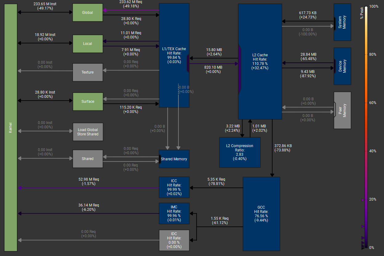
This screenshot shows the CUDA memory performance before and after the alignment fix. Notice how the number of global memory requests dropped significantly, leading to better cache utilization and reduced memory traffic. The only difference is that Vec3 is aligned to 16 bytes.
Global Memory Performance
| Metric | Before | After | Improvement |
|---|---|---|---|
| Global Memory Requests | ~459.68M requests | ~233.62M requests | -226.06M (-50.08%) |
| Frame Time | ~10 ms | ~8 ms | ~ -2 ms ~(-20%) |
Alternatively, switch to glm::vec4 if the extra float isn't a concern. The key
is
making sure each element of your
data layout is 16-byte aligned, especially if you access it frequently inside inner
loops.
CUDA's memory subsystem heavily favors aligned and coalesced reads. Without alignment, even perfect data layouts can suffer from doubled memory traffic. With alignment, you get fewer loads and fewer cacheline splits.
Gotcha: Float16 and Half Precision
I also experimented with writing my own math types to enforce alignment, and even
tested
alternatives
like using
__half to reduce memory bandwidth. However, these experiments yielded
no
measurable
performance gain.
On older NVIDIA architectures (e.g. Turing), half-precision could offer up to 2x the
FLOPs
compared
to full-precision,
but on Ampere and beyond (which is what I'm running on), FP16 and
FP32 CUDA
core
throughput
is equivalent. So, using __half didn't help—and added complexity
instead.
Opt #10 — Using Constant Memory Instead of Global Memory
One of the most effective register-saving optimizations in CUDA is proper use of the
__constant__ memory space.
This is especially beneficial when dealing with per-frame parameters that:
- Change infrequently (typically once per frame).
- Are read-only from the kernel's perspective.
- Are accessed uniformly across threads in a warp (broadcast access).
In my path tracer, I created a RenderParams structure that encapsulates all such
parameters:
struct RenderParams
{
    Hitables::PrimitiveList* __restrict__ List {};
    BVH::BVHSoA* __restrict__ BVH {};
    Mat::Materials* __restrict__ Materials {};
    uint32_t* __restrict__ RandSeeds {};
    CameraPOD Camera {};
    float4    ResolutionInfo {}; // x: x Pixel Size, y: y Pixel Size, z: width, w: height
    cudaSurfaceObject_t Image {};
    uint32_t m_SamplesPerPixel {};
    uint32_t m_MaxDepth {};
    float    m_ColorMul {};
};
Constant memory on CUDA devices is a small (typically 64 KB) memory region optimized for broadcast access. When every thread in a warp reads the same address from constant memory, the value is broadcast efficiently to all threads. This is ideal for things like camera parameters, resolution information, and control settings that are used consistently by every thread.
What makes this optimization powerful is that:
- The compiler doesn't allocate registers for constant values — they are referenced directly.
- There's no need to pass many arguments through kernel parameters, avoiding register pressure from parameter passing.
- Uniform access patterns mean near-zero latency access from constant cache. Especially that they are not accessed that frequently in hot code.
This is actually how the kernel signature looked like:
__global__ void InternalRender(cudaSurfaceObject_t fb, BVHSoA* __restrict__ world, HittableList* __restrict__ list, Materials* __restrict__ materials, uint32_t max_x, uint32_t max_y, Camera* camera, uint32_t samplersPerPixel, Float colorMul, uint32_t maxDepth, uint32_t* randSeeds);My code passed such values as regular kernel arguments or global memory pointers. That forced each thread to load and hold these values separately, increasing both register pressure and global memory traffic. Now:
struct RenderParams
{
    Hitables::PrimitiveList* __restrict__ List {};
    BVH::BVH* __restrict__ BVH {};
    Mat::Materials* __restrict__ Materials {};
    uint32_t* __restrict__ RandSeeds {};
    CameraPOD			Camera {};
    float4				ResolutionInfo {}; // x: x Pixel Size, y: y Pixel Size, z: width, w: height
    cudaSurfaceObject_t Image {};
    uint32_t			m_SamplesPerPixel {};
    uint32_t			m_MaxDepth {};
    float				m_ColorMul {};
};

__constant__ inline RenderParams d_Params;
__global__ void InternalRender();
After moving the relevant data to __constant__ memory, I observed a noticeable drop in
register usage and better caching behavior. Since the
compiler knows these values are read-only and shared across all threads, it can aggressively
optimize access.
Again, I carefully chose what to place in constant memory:
- Only data that remains fixed during kernel execution (per-frame or static)
- Data accessed frequently and uniformly across all threads
- No large arrays or per-pixel/per-thread state
Examples of values that went into constant memory:
CameraPOD: used every time a ray is generatedResolutionInfo: used in every pixel calculationm_SamplesPerPixel,m_MaxDepth,m_ColorMul: constant loop bounds or scaling factors
Meanwhile, heavy or frequently written buffers (like materials or the output image) remain in global memory, passed via pointers in the constant struct, so they're still accessible efficiently but not directly stored in constant memory.
With this change, the compiler became less aggressive in spilling registers, occupancy improved, and runtime performance became more consistent — especially in large scenes with high path depth.
Shared vs Constant vs Global Memory
To clarify where constant memory fits in CUDA's memory hierarchy, here's a high-level comparison:
| Memory Type | Scope | Access Pattern | Speed | Capacity | Use Case |
|---|---|---|---|---|---|
| Constant | Global (but read-only) | Broadcast | Very Fast (cached) | 64 KB total | Uniform read-only data (e.g. parameters, transforms) |
| Shared | Per-Block | Cooperative (explicit) | Very Fast (SRAM) | Up to 100 KB per block (depending on architecture) | Thread collaboration, caching, small local working sets |
| Global | Global | Scattered | Slow (DRAM) | Many GBs | Large datasets, outputs, scene data, textures |
In simple terms:
- Use constant memory for small, uniform, read-only data that is shared across all threads.
- Use shared memory for fast, temporary per-block data, ideally when threads cooperate.
- Use global memory for everything else — especially large and frequently updated data.
In the case of my path tracer, RenderParams fits constant memory perfectly — it is
fixed across the frame, read-only, and used uniformly by all threads. This decision directly
improved performance by reducing register usage and leveraging the constant cache's broadcast
mechanism.
Opt #11 — Prefer <cmath> Intrinsics Over <algorithm>
in CUDA
When writing CUDA __device__ code, avoid using standard C++ functions like
std::max,
std::min, or std::fma. While they work on the host, they tend to produce
bloated or
inefficient PTX, leading to more global loads, predicate-based conditionals, and elevated register
pressure. In
contrast, using the float-specialized intrinsics from <cmath>—like
std::fmaxf, std::fminf, and std::fmaf—results in streamlined
hardware
instructions with significantly better performance.
Case Study: Ray-AABB Intersection
This optimization had direct impact in our BVH traversal code, where millions of ray-AABB tests are
done per
frame. Switching from the generic std::fma and std::max to the intrinsic
float versions
led to a frame time drop from 12 ms to 9 ms, and reduced
instruction
count.
// AABB intersection (optimized)
const AABB& bounds = params->BVH->m_Bounds[node.Left];
float tx0 = std::fmaf(invDir.x, bounds.Min.x, rayOriginMulNegInvDir.x);
float tx1 = std::fmaf(invDir.x, bounds.Max.x, rayOriginMulNegInvDir.x);
float ty0 = std::fmaf(invDir.y, bounds.Min.y, rayOriginMulNegInvDir.y);
float ty1 = std::fmaf(invDir.y, bounds.Max.y, rayOriginMulNegInvDir.y);
float tz0 = std::fmaf(invDir.z, bounds.Min.z, rayOriginMulNegInvDir.z);
float tz1 = std::fmaf(invDir.z, bounds.Max.z, rayOriginMulNegInvDir.z);

float tEnter = std::fmaxf(
                 std::fmaxf(std::fminf(tx0, tx1), std::fminf(ty0, ty1)),
                 std::fmaxf(std::fminf(tz0, tz1), tmin));
float tExit = std::fminf(
                std::fminf(std::fmaxf(tx0, tx1), std::fmaxf(ty0, ty1)),
                std::fminf(std::fmaxf(tz0, tz1), tmax));
bool hit = (tEnter <= tExit);
Performance Breakdown
| Function | std::fmaxf / std::fmaf |
std::max / std::fma |
|---|---|---|
| CUDA Compatibility | ✅ Built-in device intrinsics | ⚠️ May fail to compile or introduce overhead |
| PTX Output | ✅ Maps directly to FMNMX, FFMA, FMUL | ❌ Emits FSETP, FSEL, conditional branches |
| Register Pressure | ✅ Minimal | ❌ Higher due to control flow |
| NaN Behavior | ✅ IEEE 754 compliant | ❌ Inconsistent or undefined |
| Performance (in hot path) | 9 ms total frame time | 12 ms total frame time |
PTX-Level Insight
-
std::fmaxf,std::fminf,std::fmafcompile down to single-instructionFMNMX,FFMA, orFMULoperations. -
std::maxorglm::max(when not specialized) emitFSETPpredicate logic followed byFSELconditionals, increasing instruction count and divergence risks. - The generic versions can also trigger redundant loads and spills—particularly harmful in high-traffic, tight loops.
Best Practices
- Always prefer
std::fmaxf,std::fminf, andstd::fmafwhen working withfloatin CUDA. - Use
std::fmax,std::fmin, andstd::fmaonly fordouble. - Avoid
std::maxandstd::minentirely in__device__code.
Replacing generic <algorithm> utilities with <cmath>
intrinsics is
not a micro-optimization—it's a major win in performance-critical kernels. In our case, it
shaved
off
3 ms per frame and greatly simplified the PTX output.
Opt #12 — Roll Your Own RNG (LCG + Hash) Instead of curand
When working with real-time GPU workloads like path tracing, CUDA's
curand library
is often overkill. While curand provides high-quality random numbers, it incurs
substantial overhead,
including register pressure, memory footprint, and instruction complexity—none of which play well in
tight GPU loops.
Custom RNG: PCG Hash + LCG
For performance-critical use cases where statistical quality can be relaxed, combining a simple PCG-style hash with a Linear Congruential Generator (LCG) offers a great balance. This approach:
- Uses just a few integer ops
- Compiles to clean, branchless PTX
- Works in both
__host__and__device__contexts - Requires no global state or memory buffers
Code
[[nodiscard]] __device__ __host__ __forceinline__ uint32_t PcgHash(const uint32_t input)
{
    const uint32_t state = input * 747796405u + 2891336453u;
    const uint32_t word  = ((state >> ((state >> 28u) + 4u)) ^ state) * 277803737u;
    return (word >> 22u) ^ word;
}

[[nodiscard]] __device__ __host__ __forceinline__ uint32_t RandomInt(uint32_t& seed)
{
    return (seed = (1664525u * seed + 1013904223u));
}

[[nodiscard]] __device__ __host__ __forceinline__ float RandomFloat(uint32_t& seed)
{
    // Fast float generation from masked bits
    return static_cast<float>(RandomInt(seed) & 0x00FFFFFF) / static_cast<float>(0x01000000);
}

[[nodiscard]] __device__ __host__ __forceinline__ Vec2 RandomVec2(uint32_t& seed)
{
    return { RandomFloat(seed), RandomFloat(seed) };
}

[[nodiscard]] __device__ __host__ __forceinline__ Vec3 RandomVec3(uint32_t& seed)
{
    return { RandomFloat(seed), RandomFloat(seed), RandomFloat(seed) };
}
Performance Comparison
| Metric | curand | Custom RNG |
|---|---|---|
| Register Usage | ❌ High (12-16 registers per thread) | ✅ Low (2-4 registers) |
| PTX Complexity | ❌ Dozens of ops per sample | ✅ ~4-5 ALU ops per generated float |
| Global Memory | ❌ Requires setup + state buffers | ✅ Stateless, local only |
| Speed | ❌ Slower in hot paths | ✅ Fast even in tight loops |
| Randomness Quality | ✅ High (suitable for MC methods) | ⚠️ Lower (good enough for visual noise) |
When to Use
- ✅ Real-time rendering (e.g., screen-space sampling, reservoir sampling, importance sampling)
- ✅ Denoising debug masks, visualization noise
- ❌ Offline film rendering or statistical tests
In our renderer, replacing curand_uniform with this custom generator cut per-frame
execution time
by a noticeable margin. Combined with register pressure savings, it enabled tighter occupancy
and
better warp execution
in sampling-heavy shaders.
If you're hitting performance bottlenecks in CUDA sampling loops and don't need cryptographic randomness, trade entropy for speed—it's worth it.
Opt #13 — Branchless Material Sampling & Evaluation
My old implementation uses a switch over material types (Lambert, Metal,
Dielectric), each with its own
branching logic and random sampling. While straightforward, this approach incurs warp divergence,
extra branches, and duplicated work in hot inner loops.
Original Branching Version
__device__ inline bool Material::Scatter(
    const Ray& ray, const HitRecord& rec, vec3 &attenuation, Ray &scattered,
    curandState* state) const
{
    switch (m_Type) {
      case MaterialType::Lambert: { /* diffuse logic */ }
      case MaterialType::Metal:   { /* metal logic */ }
      case MaterialType::Dielectric: { /* dielectric logic */ }
    }
    return false;
}
Every ray hit executes multiple if or switch evaluations, and each path
has its own random
fetches and normalization calls—magnified millions of times per frame.
Branchless Unified Version
We replace per-material branches with a single, weighted blend of Lambert, Metal, and Dielectric contributions. Random directions, Fresnel reflectance, and face-normal tests are all computed up front, then linearly combined based on pre-normalized weights.
[[nodiscard]] __device__ __host__ CPU_ONLY_INLINE bool Scatter(Ray& ray, const HitRecord& rec, Vec3& attenuation, uint32_t& randSeed)
{
    const RenderParams* params = GetParams();

    const Vec4& albedoIor	  = params->Materials->AlbedoIOR[rec.PrimitiveIndex];
    const auto& [flags, fuzz] = params->Materials->FlagsFuzz[rec.PrimitiveIndex];

    // normalize weights
    const float sumW  = flags.x + flags.y + flags.z + 1e-6f;
    const Vec3	normW = flags / sumW;

    const Vec3 rand3 = RandomVec3(randSeed);

    // Precompute directions
    const Vec3& unitDir	   = ray.Direction; // already normalized
    const Vec3	lambertDir = glm::normalize(rec.Normal + rand3);
    const Vec3	metalRef   = reflect(unitDir, rec.Normal);
    const Vec3	metalDir   = glm::normalize(metalRef + fuzz * rand3);

    // Dielectric components using faceNormal
    const float frontFaceMask = dot(unitDir, rec.Normal) < 0.0f;
    const Vec3	faceNormal	  = frontFaceMask * rec.Normal + (1.0f - frontFaceMask) * -rec.Normal;
    const float cosTheta	  = std::fminf(dot(-unitDir, faceNormal), 1.0f);
    const float sinTheta	  = std::sqrtf(std::fmaxf(0.0f, 1.0f - cosTheta * cosTheta));
    const float etaiOverEtat  = frontFaceMask * (1.0f / albedoIor.W) + (1.0f - frontFaceMask) * albedoIor.W;
    const float cannotRefract = etaiOverEtat * sinTheta > 1.0f;
    const float reflectProb	  = cannotRefract + (1.0f - cannotRefract) * Schlick(cosTheta, albedoIor.W);
    const float isReflect	  = rand3.x < reflectProb;

    const Vec3 refracted = RefractBranchless(unitDir, faceNormal, etaiOverEtat);
    const Vec3 dielecDir = isReflect * reflect(unitDir, faceNormal) + (1.0f - isReflect) * refracted;

    // Composite direction and normalize
    const Vec3 dir = lambertDir * normW.x + metalDir * normW.y + dielecDir * normW.z;
    ray			   = Ray(rec.Location, normalize(dir));

    // Branchless attenuation: lambert & metal albedo, dielectric = 1
    const Vec3 att = reinterpret_cast<const Vec3&>(albedoIor) * (normW.x + normW.y) + Vec3(1.0f) * normW.z;
    attenuation *= att * sumW;

    // Early exit on no scatter
    const float scatterDot = dot(dir, rec.Normal);
    return (scatterDot > 0.0f) || (flags.z > 0.0f);
}
Why This Matters
- Zero material branches: All threads follow the same arithmetic path since there are no if/switch statements, so, reduced divergence.
- Single random pool: One RNG per thread, reused for all contributions.
- Blendable: Easily support mixtures of materials (e.g., layered or coated surfaces).
In my benchmarks, this branchless approach improved warp efficiency and reduced overall shader time
compared to the classic switch-based sampler,
leading to smoother
frame rates in complex scenes.
Opt #14 — Bypass CPU Staging with CUDA↔OpenGL Interop
Early on, I rendered each frame by copying the CUDA output into an sf::Image (CPU
memory), then letting SFML
upload that image to an OpenGL texture under the hood. That CPU ↔ GPU round-trip cost was small—but
measurable:
// Pseudocode of the old pipeline
cudaMemcpy(hostBuffer, deviceBuffer, size, cudaMemcpyDeviceToHost);
sf::Image img;
img.create(width, height, hostBuffer);
sf::Texture tex;
tex.update(img);  // uploads back to GPU (OpenGL context)
At 1280x720, this added about 0.2 ms of latency per frame, worth eliminating especially that it's on the CPU's side.
Solution: Direct CUDA→OpenGL Texture Mapping
By using CUDA ↔ OpenGL interop (via cudaGraphicsGLRegisterImage /
cudaGraphicsMapResources),
we can render directly into an OpenGL texture's memory, completely bypassing CPU staging:
// During init
cudaGraphicsGLRegisterImage(&cudaTexRes, glTextureID, GL_TEXTURE_2D, cudaGraphicsRegisterFlagsWriteDiscard);

// Each frame
cudaGraphicsMapResources(1, &cudaTexRes);
cudaGraphicsSubResourceGetMappedArray(&mappedArray, cudaTexRes, 0, 0);

// Render to image from kernel here...

cudaGraphicsUnmapResources(1, &cudaTexRes);

// Then simply draw the GL texture on screen
Honorable Optimization Mentions
These are optimizations I experimented with that did not yield measurable performance gains in my specific use case. However, they are worth knowing and considering in other contexts, where they may provide significant speedups.
1. __restrict__ Pointers
The __restrict__ keyword is a compiler hint that tells the compiler: "This
pointer is the only way to access the memory it points to for the duration of its
scope." This allows the compiler to make aggressive optimizations, such as reordering
memory accesses or avoiding redundant loads.
__device__ void EvaluateShading(float* __restrict__ outLuminance,
                                const float* __restrict__ normal,
                                const float* __restrict__ albedo) {
    // Implementation that assumes no aliasing between input/output pointers
}
In my case, applying __restrict__ to CUDA kernel arguments made no measurable
difference in performance, possibly because:
- My kernels already had minimal pointer aliasing.
- Access patterns were straightforward.
- The compiler may have already inferred no aliasing from the context.
Warning
⚠️ Use with caution: If you use__restrict__ and the pointers
do alias — meaning they point to overlapping memory — the compiler's optimizations
will
lead to undefined behavior and likely subtle, incorrect results.
Example of safe usage (non-aliasing):
__device__ void AddVectors(float* __restrict__ out,
                           const float* __restrict__ a,
                           const float* __restrict__ b) {
    out[0] = a[0] + b[0]; // Compiler assumes out, a, and b don't overlap
}
But what if they do alias?
// Potentially undefined behavior if a and out alias
float data[3] = {1.0f, 2.0f, 3.0f};
AddVectors(data, data, &data[1]);
// 'a' and 'out' point to overlapping memory
The compiler may optimize the load/store order assuming no aliasing (due to
__restrict__), and this can lead to incorrect results. For instance, it might cache
a[0] before realizing it was overwritten by another pointer.
This kind of subtle bug is particularly dangerous in GPU code where memory aliasing might occur implicitly due to shared memory or register reuse, and debugging is difficult.
✱ Verdict: Potentially powerful, but dangerous if misused. Use only when you're certain pointers do not alias.
2. [[likely]] and [[unlikely]] Attributes
These C++20 attributes allow you to hint to the compiler which branches are expected to be taken more often. This can help the compiler generate more optimal branch prediction layouts, reducing misprediction penalties on the CPU.
Example:
// Process leaf node
if (node.Right == UINT32_MAX) [[unlikely]]
{
    // Process hit test
    hitAnything |= Hitables::IntersectPrimitive(ray, tmin, tmax, bestHit, node.Left);

    currentNode = stackData[--stackPtr];
    continue;
}
else [[likely]]
{
    // intersect child nodes...
}
In this example, you're telling the compiler that the first branch is the common case. This might improve performance slightly on CPUs by aligning the hot path better with the CPU's instruction cache and branch predictor.
However, the actual benefit is usually small and heavily dependent on the target architecture and compiler. On GPU (e.g., CUDA), these attributes are ignored entirely by the compiler as of today.
✱ Verdict: Safe to use on CPU in hot paths with known branch probabilities. Currently no effect in CUDA. Only use when you're confident about the branch behavior.
3. Targeting Very High SM Occupancy
It's common advice in CUDA optimization to aim for high Streaming Multiprocessor (SM) occupancy, i.e., running many threads in parallel to hide memory latency. But in practice — especially for workloads like path tracing — this isn't always beneficial.
Path tracing is inherently divergent due to the randomness of rays and material scattering logic. This limits how much benefit you get from higher occupancy. When threads in the same warp take different execution paths, CUDA has to serialize their execution, which leads to reduced efficiency.
To increase occupancy (more warps in flight), I experimented with larger block sizes and different amounts of registers per thread:
| Block Size | Registers per Thread | Warps per Block | Theoretical Occupancy |
|---|---|---|---|
| 4x8 (32) | 64 | 1 | 33.3% |
| 8x8 (64) | 64 | 2 | 66.6% |
| 8x12 (96) | < 48 | 3 | 81% |
| 8x16 (128) | < 39 | 4 (Full SM) | 100% |
Conclusion
While higher theoretical occupancy—such as that achieved with 128-thread blocks—can help hide latency and improve throughput, the observed performance differences across various block sizes remained marginal. In this particular case, profiling revealed an average of only 20 active threads per warp, indicating significant warp divergence.
This divergence reduces the effective parallelism, meaning the GPU can't fully utilize its execution units, even when plenty of warps are available. As a result, simply increasing occupancy doesn't translate into better performance because:
- Warp divergence becomes a bottleneck, not occupancy.
- Instruction throughput and memory latency are only hidden if active warps are available—and in this case, many warps are partially idle.
- Optimizations like reducing register usage or maximizing block size become less impactful when execution efficiency per warp is already low.
In short, the key insight is that occupancy alone isn't enough—warp efficiency matters more. To unlock better performance, you'd likely gain more by restructuring code to minimize divergence (e.g., avoiding divergent branches inside warps) than by merely tuning block sizes or register counts.
Performance Analysis
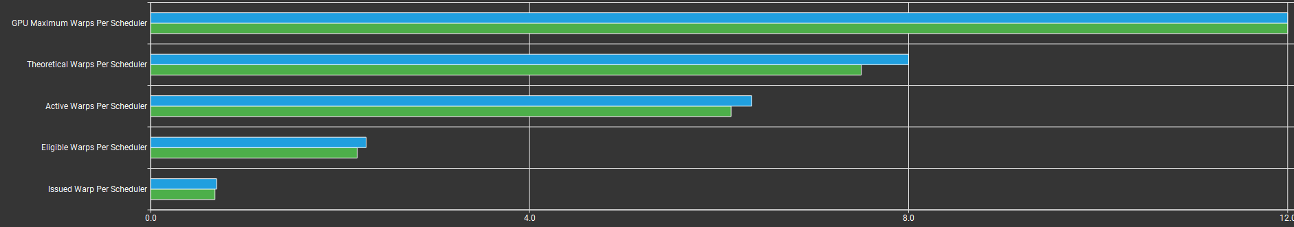
See the low Issued Warp Per Scheduler? This means that even though there are warps ready and active, very few instructions are being issued each cycle—indicating poor utilization of the scheduler's throughput.
One likely reason is that a traditional megakernel path tracer often contains complex, deeply branched logic—such as handling BVH traversal, Russian Roulette, and more—all inside a single big kernel. This causes significant warp divergence as different threads take different paths through the code.
Wavefront Path Tracing can help here by decomposing the work into separate, simpler stages (e.g., ray generation, intersection, shading). Each stage is executed by a specialized kernel operating on batches of work units that are more uniform. This means threads within a warp are more likely to follow the same execution path, dramatically improving warp efficiency and instruction issue rate.
By separating divergent logic into more uniform waves, wavefront architecture increases the likelihood that multiple instructions can be issued per cycle, improving the Issued Warp Per Scheduler metric and ultimately leading to higher overall throughput.
✱ Verdict: Don't chase maximum occupancy blindly. In divergent workloads like path tracing, higher register count and fewer threads may outperform higher occupancy configurations.
4. Van Emde Boas Layout for BVH (Post-Build Sort)
One lesser-known but promising optimization is applying a Van Emde Boas (VEB) layout to the Bounding Volume Hierarchy (BVH) as a post-processing step. The goal is to improve spatial locality, increasing the chance that memory accesses during traversal stay in the L1 cache.
In this path tracer, I'm using a Struct of Arrays (SoA) layout, which is already cache-friendly. That means each property (e.g., positions, radii, materials) is tightly packed and accessed sequentially — ideal for coalesced GPU reads.
Scene Stats:
- 488 spheres (center and radius) x sizeof(Vec4) = 7'808 bytes
- 488 materials x 2 x sizeof(Vec4) = 15'616 bytes
- 975 BVH nodes x sizeof(AABB) = 31'200 bytes
- 975 BVH nodes x sizeof(BVH node metadata) = 7'800 bytes
- Total: 62'424 bytes
Since this is well within a 256KB L1 cache, applying a VEB layout to the BVH would likely bring no meaningful performance gain in this particular case. However, in larger scenes — or if the BVH and primitives span multiple cache lines — this optimization can help reduce cache misses during traversal.
What VEB Does:
- Reorders the BVH in memory to follow a cache-oblivious, recursive layout.
- Ensures nodes accessed close together during traversal are stored close together in memory.
- Reduces memory latency and improves prefetch effectiveness on wide cache lines.
✱ Verdict: Not needed for small scenes fitting comfortably in L1 cache. But can be a big win for large, cache-stretching BVHs in real-world rendering workloads.
5. Parallelizing SAH BVH Construction
Building a Surface Area Heuristic (SAH) BVH is a key step in path tracing acceleration. While SAH construction is often viewed as expensive, it's highly parallelizable on GPUs. However, this optimization requires careful implementation and wasn't something I tackled yet.
Currently, my BVH construction is implemented recursively, which is efficient on the CPU but especially slow on GPUs due to recursion. Even stack size has to be set manually.
Interestingly, in my simple tests (single-threaded CPU vs single-threaded GPU), the CPU version was dramatically faster:
| Implementation | BVH Construction Time | Threads |
|---|---|---|
| GPU (single-threaded, recursive) | 58.694 ms | 1 |
| CPU (single-threaded, recursive) | 0.829 ms | 1 |
This result shocked me — CPUs have advanced scalar cores with sophisticated branch prediction and fast caches that make single-threaded SAH extremely efficient. Meanwhile, GPU SAH builds without parallelization and using recursion struggle significantly.
Takeaway: SAH BVH construction can be massively accelerated on the GPU with well-designed parallel and iterative algorithms. It's a worthy optimization for future work but requires rewriting recursive parts and handling GPU-specific challenges like thread divergence and memory management.
✱ Verdict: Great potential but complex. Worth exploring if BVH build times become a bottleneck.
Results And Benchmarks
To verify the performance of my CUDA ray tracer across different systems and resolutions, I ran a standardized benchmark using a fixed camera view and identical rendering settings across devices:
- Resolutions: 1280x720, 1920x1080, 2560x1440, and 3840x2160
- Samples per pixel: 30
- Max ray depth: 50
- Benchmarking duration: Single frame (no accumulation over time)
- Measurement method on GPU:
cudaEventRecordaround the entire rendering kernel - Measurement method on CPU:
std::steady_clock::now()around the entire rendering code
Nsight Compute Results
These are from my RTX 3080 run if you'd like to explore the kernel analysis yourself.
| Nsight Compute Report | Frame Time | Download Link |
|---|---|---|
| Old/Slow | 2380 ms | Download Old Report (.ncu-rep) |
| Latest/Improved | 8 ms | Download Latest Report (.ncu-rep) |
benchmark Results
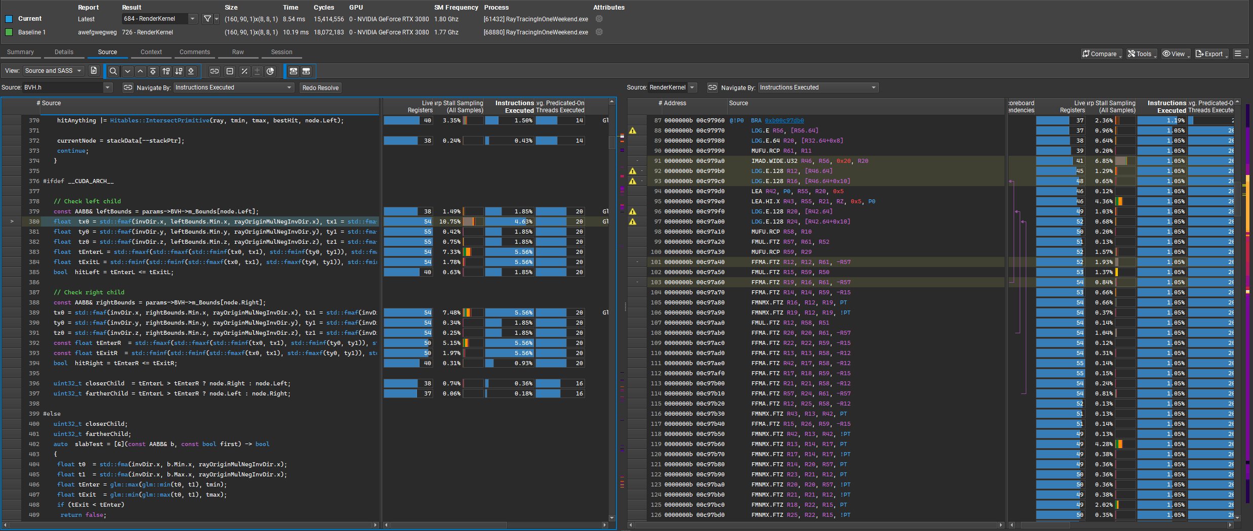
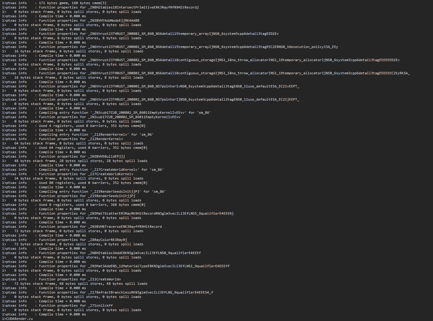
The SASS instructions in the image are mostly FFMA, FMUL, and FMNMX—fast math operations ideal for compute-bound CUDA kernels. This shows the ray tracing inner loops are efficiently mapped to hardware, with minimal branching or memory stalls. Most stalls are not memory-related but due to scheduler choices or instruction dependencies. This efficient math mapping is a direct result of the described optimizations and explains the significant speedup in the final benchmarks.
Below are the measured frame times in milliseconds. Lower is better:
| GPU / CPU | 1280x720 | 1920x1080 | 2560x1440 | 3840x2160 |
|---|---|---|---|---|
| RTX 3080 | 9.12 ms | 19.5 ms | 35 ms | 76 ms |
| i5-13600KF | 450 ms | 980 ms | 1770 ms | 3845 ms |
| RTX 3050 Laptop | 27 ms | 53 ms | 115 ms | 256 ms |
| i5-13450HX | 1000 ms | 2250 ms | 4565 ms | 10350 ms |
| RTX 4050 Laptop | 20 ms | 40 ms | 75 ms | 165 ms |
| i7-13700H | 725 ms | 1450 ms | 2675 ms | 8284 ms |
As expected, GPU acceleration dominates here—especially on higher-end GPUs like the RTX 3080, where even 4K renders finish in under 80ms. The gap between CUDA and CPU-only performance is dramatic, often exceeding 50x at higher resolutions.
Laptops with mid-range GPUs like the RTX 3050 and 4050 also deliver playable performance in 1080p, while CPUs struggle even at lower resolutions.
Future Work
As with any graphics project, there's always something cooler, faster, or more unnecessarily complicated to try. Here's what's on my radar for future exploration:
🌊 Wavefront Path Tracing
Traditional megakernels—like the one I'm currently using—tend to suffer from high register pressure, warp divergence, and other GPU ailments. Wavefront path tracing offers a remedy by breaking the pipeline into separate, parallel stages (generate rays, intersect, shade, etc.), which allows better control over occupancy and divergence.
There's compelling evidence that wavefront is significantly faster under the right conditions:
Reddit
discussion on wavefront being 5x faster
And a solid academic backbone from NVIDIA Research:
Megakernels
Considered Harmful — Laine & Karras
It's not trivial to implement—requires work queues, persistent kernels, and possibly a mild existential crisis—but it's one of the best-known performance unlocks for complex scenes.
📐 Triangle Support via TinyBVH?
While my current path tracer only supports spheres (like it's still 2004), the next logical step is supporting triangle geometry. I'm exploring tinybvh for fast triangle BVH construction and traversal.
This will open the door to loading full mesh scenes (like Cornell Boxes and Sponza), potentially with hardware-accelerated triangle intersection via CUDA intrinsics.
💥 OptiX Backend
Eventually, I'd like to compare this CUDA implementation with an OptiX-based path tracer. That would allow testing hardware ray tracing (RT cores) vs. our current software traversal, and take advantage of the mature BVH traversal stack in OptiX.
💼 Also... I'm Looking for a Job 😅
If you've made it this far, first of all: respect. Second of all, hey—I'm actively looking for a role in graphics programming, CUDA/GPU engineering, or real-time rendering. So if you're a hiring manager, let's talk. Check my resume, or just shoot me a message. I'll even throw in a free bug fix.
References
-
Ray
Tracing in One Weekend
by Peter Shirley
A classic introductory book series that helped shape the structure of my path tracer. Available freely at: -
GPSnoopy's
RayTracingInVulkan
A well-structured real-time ray tracing renderer in Vulkan with RTX support. -
NVIDIA CUDA
Programming Guide
The definitive guide for CUDA architecture, performance tips, and memory behavior. Especially useful for understanding occupancy, warp scheduling, and function inlining. -
Optimizing CUDA by Nvidia
DevBlog
Multiple performance blog posts from NVIDIA covering best practices, launch configuration, memory coalescing.. -
RTX Best Practices — NVIDIA Developer Blog
NVIDIA's official guide to best practices for real-time ray tracing with RTX, including performance tips and architectural insights. -
Accelerated
Ray
Tracing in CUDA — NVIDIA Developer Blog
A practical overview on implementing ray tracing using CUDA, including memory layout, BVH traversal, and shading strategies. -
NVIDIA Ampere GA102 GPU Architecture Whitepaper (PDF)
A valuable source when it comes to architecture-specific optimizations. It says FP16(non-Tensor) runs at full speed as FP32 on the Ampere architecture.
Always compile with
-Xptxas=-vThis will show information about each compiled function-how many register? how many bytes spilled to memory, how big is the stack frame?
Use Nsight Compute's built-in occupancy calculator!
This is really useful, you give information about your kernel, it tells you what's actually limiting your occupancy, neat!